


(published May 2012)
In many inland waters, tidal current flow is a dominating factor in navigation. In special cases like the Gulf Stream, it can also be crucial in the ocean. With a working GPS, it is less of a challenge once underway because we can see directly from our recorded track across an e-chart whether or not we are getting set off of our desired course line. If we are getting set off, we can steer into the current to get back onto our desired course line and then correct for the set to stay on this line. All of which assumes we have such options! Under sail, we do not have this option going to weather, but sometimes do on other points of sail. In any event, what we will cover here can be useful even if we can’t correct for it.
In principle, the amount you correct is not the same as the amount you are getting set, but this is always a good starting point. If I am steering 300 and getting set to 320, then my first guess is to steer 280 to make good 300. But we always want to fine-tune this to get it right. It could be that an average of 283 makes good 300, but by the time you learn that, you are well off your course line (waypoint to waypoint). So overcorrect to get back on the line, and then come back to 283. Good navigation means choosing the right waypoints in the first place, then sailing waypoint to waypoint, staying on your intended line. In the presence of underwater hazards this is absolutely crucial, but it is always good policy. Otherwise you are not navigating—you are just out sailing.
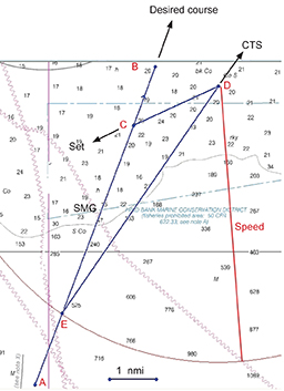
1. Draw line AB in the direction of your desired course.
2. At any point C, extend your current vector back into the current, length = drift, direction = set + 180, with line CD.
3. From point D, swing an arc of length = knotmeter speed so as to intersect AB at point E.
4. Then direction ED = CTS to make good your desired course, and EC will be your SMG.
In other words, in one hour you move from E to D and in that same hour the water moves from D to C, so you are actually progressing from E to C along your desired course but in this case (current forward of the beam) you will be making good a slower speed than your knotmeter speed.
This numerical example is for S=6, desired course = 020, set =
245 and drift = 2. The plotted solution here yields CTS = 033.6 and SMG = 4.4. The correction angle = 033.6 – 020.0 = 13.6°. If we use our trick formula, we get set = correction = (2/6)x40° = 13.3°, which only goes to show that it is not often we need to bring out these big guns!
Since we know we can’t always correct for the current under sail, it pays to think through the effect of the current before we leave. This prepares us for the magnitude of the effects we can’t control, as well as making the adjustments more understandable when we can make them. Over the years we have developed several tricks and procedures at Starpath School of Navigation that make this job easier and more accurate.
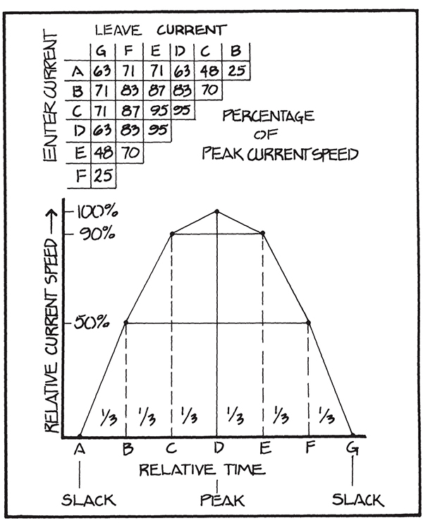
One trick, the “Starpath 50-90 Rule,” can be used to predict current speeds in between slack and peak flow. A typical tidal current cycle goes from slack water to peak flow and back to slack water in some four to seven hours, with the average being about six hours. Thus, we divide the cycle from slack to peak into three equal time intervals, as shown in Figure 1. On a world average, the intervals would be about one hour each, but using thirds makes it more universal. Thus the rule is that the current rises from slack to 50% of its peak in the first third, then to 90% in the second third, and finally to its peak in the last third. It is a way to approximate current speed at intermediate times for typical reversing tidal currents. The US Power Squadron has adopted this rule and offers work forms for applying it.
There are tables and diagrams in the NOAA Current Tables for figuring the intermediate speeds, but this rule is easier to remember and apply. Also, strong currents in very constricted passes can rise and fall more quickly than this (called a hydraulic head). Such currents are usually noted in the current tables with a special intermediate speed table.
Once we have a way to estimate a current at any time, we can make the correction for it either properly with a vector plot as shown in Figure 2, or we can use our trick for figuring it out in our heads (shown in Figure 3). The estimate makes several math approximations, in addition to the basic assumption that the correction equals the amount we get set. In other words, this trick is telling us how much we get set if we do nothing, and we just assume we will go straight if we point into the current by the same amount. In practical navigation these estimates are good enough because we do not know the currents well enough to justify a proper solution.
The third procedure to share here is our method of estimating the effective average current if we spend some time within a changing current pattern. In other words, what is the effective average current if we enter at one point in the cycle and leave at another? This important factor can be readily figured from the insert to Figure 1.
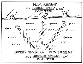
At a knotmeter speed of 6 kts crossing a 2-kt current on the beam, the set angle (α) is (2/6) x 60° = 20°.
This same current on the bow or quarter would call for a correction of (2/6) x 40° = 13°.
Picture and method reproduced from Inland and Coastal Navigation by David Burch (www.starpathpublications.com)
As an example, consider a current crossing without GPS. Current tables tell us the current sets due west (flows toward 270 T); it is slack at 0900, and has a peak of 2.0 kts at 1200. Our destination is 5 nm off in direction 045 T. Our knotmeter speed is 5.0 kts. We will be leaving at 10 a.m. What correction would we make to our course to get there on a single heading?
A first estimate of the crossing time would be one hour, thus from Figure 1 we enter the current at B and leave at C, which gives us a net average current of 0.70 x 2.0 = 1.4 kts. Our quick estimate of the set from Figure 3 would be (1.4 / 5.0) x 40° = 11.2°. Thus we should sail 11° into the current (new course 056 T) to get to our destination on one constant heading. On this course we would first be overcorrecting, then later undercorrecting and end up on target. Not ideal since we wander off our track, but easy to figure on the wing. In waterways with hazards, we would want to break the trip up into smaller legs to stay closer to the intended track line. In any event, the diagrams provide the solution to any number of steps.
If we plot this out more accurately with the method in Figure 2, the mathematically correct heading is 056.4° and the resulting speed made good (SMG) would be 3.91 kts. Our trick for figuring set angle does not give us SMG, but for currents on the bow or beam, the SMG is less than knotmeter speed, and for quarter currents it is faster.
David Burch is the director of Starpath School of Navigation, which offers online courses in marine navigation and weather at www.starpath.com. He has written eight books on navigation and received the Institute of Navigation’s Superior Achievement Award for outstanding performance as a practicing navigator. David will answer questions about the article or other matters of navigation at facebook.com/starpathnav